60. 卷积神经网络构建

60.1. 介绍

前面，我们已经学习了卷积神经网络的原理，尤其对卷积层和池化层等关键组件进行了详细说明。本次实验会关注于如何利用深度学习框架构建卷积神经网络，并完成模型训练。

60.2. 知识点

• TensorFlow 高阶 API 构建

• TensorFlow 低阶 API 构建

• PyTorch 低阶 API 构建

• PyTorch 高阶 API 构建

前面的实验已经学习了如何使用 TensorFlow 和 PyTorch 搭建人工神经网络并完成训练。实际上，构建卷积神经网络的流程和全连接神经网络别无二致，区别仅在于向神经网络中添加卷积神经网络所需的特殊组件。

接下来，实验将尝试使用前面学过的 4 种方法来搭建一个卷积神经网络，其分别是：TensorFlow 低阶 tf.nn 模块和高阶 tf.keras 模块，以及 PyTorch 模块 nn.Module 和 nn.Sequential。

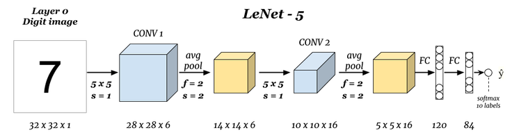
实验仍然使用大家熟悉的 MNIST 数据集，该数据集样本数量适中，非常适合用于练习。神经网络则选择 Yann LeCun 在 1998 年发明的 LeNet-5 经典卷积神经网络结构。

来源

60.3. 数据预处理

对于 MNIST 数据集，我们已经分别使用 TensorFlow 和 PyTorch 加载过。实际上，深度学习框架加载数据集的 API 是直接从 LeCun 的网站 上下载相应的数据集。这里，我们下载镜像文件。

# 直接运行下载数据文件
wget -nc "https://cdn.aibydoing.com/hands-on-ai/files/MNIST_data.zip"
unzip -o "MNIST_data.zip"

文件 “MNIST_data.zip” 已经存在；不获取。

Archive:  MNIST_data.zip
 extracting: MNIST_data/t10k-labels-idx1-ubyte.gz  
 extracting: MNIST_data/train-labels-idx1-ubyte.gz  
  inflating: MNIST_data/t10k-images-idx3-ubyte.gz  
  inflating: MNIST_data/train-images-idx3-ubyte.gz  

数据集一共包含四个文件，分别是：

• 训练样本：train-images-idx3-ubyte.gz

• 训练标签：train-labels-idx1-ubyte.gz

• 测试样本：t10k-images-idx3-ubyte.gz

• 测试标签：t10k-labels-idx1-ubyte.gz

数据使用 IDX 文件格式存储，首先需要将其读取出来。

# 此段数据读取代码无需掌握
import gzip
import numpy as np


def read_mnist(images_path, labels_path):
    with gzip.open("MNIST_data/" + labels_path, "rb") as labelsFile:
        y = np.frombuffer(labelsFile.read(), dtype=np.uint8, offset=8)

    with gzip.open("MNIST_data/" + images_path, "rb") as imagesFile:
        X = (
            np.frombuffer(imagesFile.read(), dtype=np.uint8, offset=16)
            .reshape(len(y), 784)
            .reshape(len(y), 28, 28, 1)
        )

    return X, y


train = {}
test = {}

train["X"], train["y"] = read_mnist(
    "train-images-idx3-ubyte.gz", "train-labels-idx1-ubyte.gz"
)
test["X"], test["y"] = read_mnist(
    "t10k-images-idx3-ubyte.gz", "t10k-labels-idx1-ubyte.gz"
)

train["X"].shape, train["y"].shape, test["X"].shape, test["y"].shape

((60000, 28, 28, 1), (60000,), (10000, 28, 28, 1), (10000,))

可以看到，训练集 60000 个，图像为 \(28 \times 28\) 大小，其中灰度图像保留色彩通道 1。测试集包含 10000 个样本。我们可以可视化第一个样本。

from matplotlib import pyplot as plt

%matplotlib inline

plt.imshow(train["X"][0].reshape(28, 28), cmap=plt.cm.gray_r)

<matplotlib.image.AxesImage at 0x13e380100>

返回上面 LeNet-5 网络结构示意图，你会看到原始的 LeNet-5 结构输入图像尺寸为 32x32x1。所以，我们这里的数据预处理尚未结束，可以通过向 28x28x1 的图像外圈各填充 2 个 0 值来达到效果，这样就可以分毫不差地实现 LeNet-5 卷积神经网络了。

同时，由于 LeNet-5 最终是 Softmax 输出，所以我们需要对标签进行独热编码处理，这一步已经在前面的实验中学习过了。

# 样本 padding 填充
X_train = np.pad(train["X"], ((0, 0), (2, 2), (2, 2), (0, 0)), "constant")
X_test = np.pad(test["X"], ((0, 0), (2, 2), (2, 2), (0, 0)), "constant")
# 标签独热编码
y_train = np.eye(10)[train["y"].reshape(-1)]
y_test = np.eye(10)[test["y"].reshape(-1)]

X_train.shape, X_test.shape, y_train.shape, y_test.shape

((60000, 32, 32, 1), (10000, 32, 32, 1), (60000, 10), (10000, 10))

我们可以再次通过可视化确认修改。

from matplotlib import pyplot as plt

%matplotlib inline

plt.imshow(X_train[0].reshape(32, 32), cmap=plt.cm.gray_r)

<matplotlib.image.AxesImage at 0x13e44a0e0>

60.4. TensorFlow 高阶 tf.keras 构建

由于高阶 API 使用起来更加简单，所以我们首先使用 TensorFlow 提供的 Keras 来构建 LeNet-5 卷积神经网络。在这之前，需要先了解需要用到的卷积层和池化层。

其中，tf.keras.layers 🔗 下包含的卷积层类有：

• tf.keras.layers.Conv1D 🔗：一般用于文本或时间序列上的一维卷积。

• tf.keras.layers.Conv2D 🔗：一般用于图像空间上的二维卷积。

• tf.keras.layers.Conv3D 🔗。一般用于处理视频等包含多帧图像上的三维卷积。

关于 3 者详细区别可以阅读 Intuitive understanding… 实际上，我们在图像处理方面一般只会用到 tf.keras.layers.Conv2D。

卷积层类包含的参数很多，不过我们一般用到的无外乎就是：

• filters: 卷积核数量，整数。

• kernel_size: 卷积核尺寸，元组。

• strides: 卷积步长，元组。

• padding: "valid" 或 "same"。

特别注意，如果卷积层在模型第一层时，需要提供 input_shape 参数，例如，input_shape=(128, 128, 3) 表示 128x128 RGB 图像。此时，会关联上一个默认参数 data_format="channels_last"，也就是色彩通道数量 3 在最后。当然，如果你的 input_shape=(3, 128, 128)，就需要指定参数 data_format="channels_first"。

其次，需要说明的是 padding 支持两个参数，分别是 "valid" 或 "same"（大小写敏感）。下面说一下这两个参数在 TensorFlow 中的含义。假设，输入矩阵的一行如下所示，包含 13 个单位。

当参数为 "valid" 时（默认），无法被卷积的像素将被丢弃。也就是不会对边距进行扩充，相当于不需要 Padding 操作。

当参数为 "same" 时，将通过 0 填补保证每一个输入像素都能被卷积。

如上所示，通过添加 3 个为 0 的格子保证每一个输入像素都能被卷积。添加时，如果遇到上面这种奇数的情况，默认在右边会更多。

除此之外，池化层在图像处理时一般也只会用到带 2D 的类，例如 LeNet-5 网络中需要的平均池化 tf.keras.layers.AveragePooling2D 🔗。

池化层中常用的 2 个参数：pool_size 和 stride。pool_size 池化窗口默认为 (2, 2)，也就是将张量缩减为原来尺寸的一半大小。stride 表示缩小比例的因数，例如，2 会使得输入张量缩小一半。 如果是 None，那么默认值是 pool_size。

来源

下面，我们使用 TensorFlow 提供的 Keras 高阶 API 来构建 LeNet-5 卷积神经网络。除了如图所示的已知参数以外，像卷积核数量，激活函数等参考原论文提供的数据指定。

import tensorflow as tf

model = tf.keras.Sequential()  # 构建顺序模型

# 卷积层，6 个 5x5 卷积核，步长为 1，relu 激活，第一层需指定 input_shape
model.add(
    tf.keras.layers.Conv2D(
        filters=6,
        kernel_size=(5, 5),
        strides=(1, 1),
        activation="relu",
        input_shape=(32, 32, 1),
    )
)
# 平均池化，池化窗口默认为 2
model.add(tf.keras.layers.AveragePooling2D(pool_size=(2, 2), strides=2))
# 卷积层，16 个 5x5 卷积核，步为 1，relu 激活
model.add(
    tf.keras.layers.Conv2D(
        filters=16, kernel_size=(5, 5), strides=(1, 1), activation="relu"
    )
)
# 平均池化，池化窗口默认为 2
model.add(tf.keras.layers.AveragePooling2D(pool_size=(2, 2), strides=2))
# 需展平后才能与全连接层相连
model.add(tf.keras.layers.Flatten())
# 全连接层，输出为 120，relu 激活
model.add(tf.keras.layers.Dense(units=120, activation="relu"))
# 全连接层，输出为 84，relu 激活
model.add(tf.keras.layers.Dense(units=84, activation="relu"))
# 全连接层，输出为 10，Softmax 激活
model.add(tf.keras.layers.Dense(units=10, activation="softmax"))
# 查看网络结构
model.summary()

Model: "sequential"
_________________________________________________________________
 Layer (type)                Output Shape              Param #   
=================================================================
 conv2d (Conv2D)             (None, 28, 28, 6)         156       
                                                                 
 average_pooling2d (Average  (None, 14, 14, 6)         0         
 Pooling2D)                                                      
                                                                 
 conv2d_1 (Conv2D)           (None, 10, 10, 16)        2416      
                                                                 
 average_pooling2d_1 (Avera  (None, 5, 5, 16)          0         
 gePooling2D)                                                    
                                                                 
 flatten (Flatten)           (None, 400)               0         
                                                                 
 dense (Dense)               (None, 120)               48120     
                                                                 
 dense_1 (Dense)             (None, 84)                10164     
                                                                 
 dense_2 (Dense)             (None, 10)                850       
                                                                 
=================================================================
Total params: 61706 (241.04 KB)
Trainable params: 61706 (241.04 KB)
Non-trainable params: 0 (0.00 Byte)
_________________________________________________________________

你可以看到，网络结构与图示完成一致。接下来，我们就可以编译模型并完成训练和评估了。

# 编译模型，Adam 优化器，多分类交叉熵损失函数，准确度评估
model.compile(optimizer="adam", loss="categorical_crossentropy", metrics=["accuracy"])

# 模型训练及评估
model.fit(X_train, y_train, batch_size=64, epochs=2, validation_data=(X_test, y_test))

Epoch 1/2
938/938 [==============================] - 6s 7ms/step - loss: 0.3219 - accuracy: 0.9330 - val_loss: 0.0781 - val_accuracy: 0.9752
Epoch 2/2
938/938 [==============================] - 6s 6ms/step - loss: 0.0668 - accuracy: 0.9796 - val_loss: 0.0607 - val_accuracy: 0.9813

<keras.src.callbacks.History at 0x290564c10>

60.5. TensorFlow 低阶 tf.nn 构建

TensorFlow 低阶 API 主要会用到 tf.nn 模块，通过构建前向计算图后，再建立会话完成模型训练。其中，卷积函数为 tf.nn.conv2d 🔗，平均池化函数为 tf.nn.avg_pool 🔗。值得注意的是，虽然大部分参数含义上和 Keras 相似，但是用法上却不同，大家需要根据下面的示例代码并结合官方文档学习。

当我们使用 tf.nn 实现时，就需要像先前的全连接神经网络一样自行初始化权值（卷积核），这里可以利用 random_normal 按照给定任意的矩阵大小，随机生成权重数值。

class Model(object):
    def __init__(self):
        # 随机初始化张量参数
        self.conv_W1 = tf.Variable(tf.random.normal(shape=(5, 5, 1, 6)))
        self.conv_W2 = tf.Variable(tf.random.normal(shape=(5, 5, 6, 16)))
        self.fc_W1 = tf.Variable(tf.random.normal(shape=(5 * 5 * 16, 120)))
        self.fc_W2 = tf.Variable(tf.random.normal(shape=(120, 84)))
        self.out_W = tf.Variable(tf.random.normal(shape=(84, 10)))

        self.fc_b1 = tf.Variable(tf.zeros(120))
        self.fc_b2 = tf.Variable(tf.zeros(84))
        self.out_b = tf.Variable(tf.zeros(10))

    def __call__(self, x):
        x = tf.cast(x, tf.float32)  # 转换输入数据类型
        # 卷积层 1: Input = 32x32x1. Output = 28x28x6.
        conv1 = tf.nn.conv2d(x, self.conv_W1, strides=[1, 1, 1, 1], padding="VALID")
        # RELU 激活
        conv1 = tf.nn.relu(conv1)
        # 池化层 1: Input = 28x28x6. Output = 14x14x6.
        pool1 = tf.nn.avg_pool(
            conv1, ksize=[1, 2, 2, 1], strides=[1, 2, 2, 1], padding="VALID"
        )
        # 卷积层 2: Input = 14x14x6. Output = 10x10x16.
        conv2 = tf.nn.conv2d(pool1, self.conv_W2, strides=[1, 1, 1, 1], padding="VALID")
        # RELU 激活
        conv2 = tf.nn.relu(conv2)
        # 池化层 2: Input = 10x10x16. Output = 5x5x16.
        pool2 = tf.nn.avg_pool(
            conv2, ksize=[1, 2, 2, 1], strides=[1, 2, 2, 1], padding="VALID"
        )
        # 展平. Input = 5x5x16. Output = 400.
        flatten = tf.reshape(pool2, [-1, 5 * 5 * 16])
        # 全连接层
        fc1 = tf.nn.relu(tf.add(tf.matmul(flatten, self.fc_W1), self.fc_b1))
        fc2 = tf.nn.relu(tf.add(tf.matmul(fc1, self.fc_W2), self.fc_b2))
        outs = tf.add(tf.matmul(fc2, self.out_W), self.out_b)
        return outs

接下来的流程和之前使用 TensorFlow 完成 DIGITS 分类非常相似了。分别定义损失函数和准确度计算函数。

def loss_fn(model, x, y):
    preds = model(x)
    return tf.reduce_mean(
        tf.nn.softmax_cross_entropy_with_logits(logits=preds, labels=y)
    )

def accuracy_fn(logits, labels):
    preds = tf.argmax(logits, axis=1)  # 取值最大的索引，正好对应字符标签
    labels = tf.argmax(labels, axis=1)
    return tf.reduce_mean(tf.cast(tf.equal(preds, labels), tf.float32))

如果我们使用 TensorFlow 低阶 API 构建神经网络，那么就需要自行实现小批量训练过程，以防止一次传入数据太多导致内存爆掉。同样，这部分代码在先前的实验中也已经实现过了，所以我们直接拿过来修改合适的迭代次数和小批量大小即可。

from sklearn.model_selection import KFold
from tqdm.notebook import tqdm

EPOCHS = 2  # 迭代此时
BATCH_SIZE = 64  # 每次迭代的批量大小
LEARNING_RATE = 0.001  # 学习率

model = Model()  # 实例化模型类

for epoch in range(EPOCHS):  # 设定全数据集迭代次数
    indices = np.arange(len(X_train))  # 生成训练数据长度规则序列
    np.random.shuffle(indices)  # 对索引序列进行打乱，保证为随机数据划分
    batch_num = int(len(X_train) / BATCH_SIZE)  # 根据批量大小求得要划分的 batch 数量
    kf = KFold(n_splits=batch_num)  # 将数据分割成 batch 数量份
    # KFold 划分打乱后的索引序列，然后依据序列序列从数据中抽取 batch 样本
    for _, index in tqdm(kf.split(indices), desc="Training"):
        X_batch = X_train[indices[index]]  # 按打乱后的序列取出数据
        y_batch = y_train[indices[index]]

        with tf.GradientTape() as tape:  # 追踪梯度
            loss = loss_fn(model, X_batch, y_batch)

        trainable_variables = [
            model.conv_W1,
            model.conv_W2,
            model.fc_W1,
            model.fc_W2,
            model.out_W,
            model.fc_b1,
            model.fc_b2,
            model.out_b,
        ]  # 需优化参数列表
        grads = tape.gradient(loss, trainable_variables)  # 计算梯度

        optimizer = tf.optimizers.Adam(learning_rate=LEARNING_RATE)  # Adam 优化器
        optimizer.apply_gradients(zip(grads, trainable_variables))  # 更新梯度

    # 每一次 Epoch 执行小批量测试，防止内存不足
    indices_test = np.arange(len(X_test))
    batch_num_test = int(len(X_test) / BATCH_SIZE)
    kf_test = KFold(n_splits=batch_num_test)
    test_acc = 0
    for _, index in tqdm(kf_test.split(indices_test), desc="Testing"):
        X_test_batch = X_test[indices_test[index]]
        y_test_batch = y_test[indices_test[index]]
        batch_acc = accuracy_fn(model(X_test_batch), y_test_batch)  # 计算准确度
        test_acc += batch_acc  # batch 准确度求和

    accuracy = test_acc / batch_num_test  # 测试集准确度
    print(f"Epoch [{epoch+1}/{EPOCHS}], Accuracy: [{accuracy:.2f}], Loss: [{loss:.4f}]")

Epoch [1/2], Accuracy: [0.89], Loss: [25219.9238]

Epoch [2/2], Accuracy: [0.91], Loss: [12266.0176]

你可能会发现同样的网络结构我们使用 Keras 得到的效果会更好一些。实际上，这就是使用高阶 API 的好处，其在学习率，权重初始化等细节方面已经得到充分优化。所以，一般情况下能用 TensorFlow 高阶 API 搭建的网络，我们就不会使用低阶 API 自找麻烦。不过低阶 API 又更灵活，可以满足高级开发者或者学术研究人员的需要。

60.6. PyTorch 低阶 nn.Module 构建

我们已经使用 TensorFlow 提供的 2 种常用流程构建了 LeNet-5 卷积神经网络完成 MNIST 训练。接下来，实验使用 PyTorch 提供的 API 来重构 LeNet-5 的整个过程。

首先，我们基于 nn.Module 来构建神经网络。还记得吗？这里需要继承 nn.Module 基类来实现自定义神经网络结构。

import torch
import torch.nn as nn
import torch.nn.functional as F


class LeNet(nn.Module):
    def __init__(self):
        super(LeNet, self).__init__()
        # 卷积层 1
        self.conv1 = nn.Conv2d(
            in_channels=1, out_channels=6, kernel_size=(5, 5), stride=1
        )
        # 池化层 1
        self.pool1 = nn.AvgPool2d(kernel_size=(2, 2))
        # 卷积层 2
        self.conv2 = nn.Conv2d(
            in_channels=6, out_channels=16, kernel_size=(5, 5), stride=1
        )
        # 池化层 2
        self.pool2 = nn.AvgPool2d(kernel_size=(2, 2))
        # 全连接层
        self.fc1 = nn.Linear(in_features=5 * 5 * 16, out_features=120)
        self.fc2 = nn.Linear(in_features=120, out_features=84)
        self.fc3 = nn.Linear(in_features=84, out_features=10)

    def forward(self, x):
        x = F.relu(self.conv1(x))
        x = self.pool1(x)
        x = F.relu(self.conv2(x))
        x = self.pool2(x)
        x = x.reshape(-1, 5 * 5 * 16)
        x = F.relu(self.fc1(x))
        x = F.relu(self.fc2(x))
        x = F.softmax(self.fc3(x), dim=1)
        return x

值得注意的是，PyTorch 中卷积层参数与 TensorFlow 有别。PyTorch 没有 TensorFlow 中卷积核数量的参数，取而代之需要设定 out_channels 来代之卷积核数量。其实也很好理解，in_channels 个通道的图像输出传出 out_channels 个通道，自然也是通过 out_channels 个卷积核进行了处理。

池化层和全连接层应该很好理解。特别地，PyTorch 中没有 Flatten 展平层相关类，所以我们在网络中使用 x.reshape(-1, 5*5*16) 将张量转换为我们需要的形状。

下面，实例化自定义模型类，打印出模型结构。

model = LeNet()
model

LeNet(
  (conv1): Conv2d(1, 6, kernel_size=(5, 5), stride=(1, 1))
  (pool1): AvgPool2d(kernel_size=(2, 2), stride=(2, 2), padding=0)
  (conv2): Conv2d(6, 16, kernel_size=(5, 5), stride=(1, 1))
  (pool2): AvgPool2d(kernel_size=(2, 2), stride=(2, 2), padding=0)
  (fc1): Linear(in_features=400, out_features=120, bias=True)
  (fc2): Linear(in_features=120, out_features=84, bias=True)
  (fc3): Linear(in_features=84, out_features=10, bias=True)
)

很遗憾，PyTorch 并无法像 TensorFlow 那样打印出模型间张量尺寸的变化，不过你可以借助 Model summary in PyTorch 等第三方工具实现。实验中不再尝试。

下面，我们对模型进行测试，输入一个样本张量看一下能否正常在自定义模型间进行计算，且输出形状是否符合预期。当我们取出第一个样本 X_train[0] 时，其形状为 (32, 32, 1)。这并不符合 PyTorch 样本传入形状。我们需要按照 PyTorch 的特性，将样本转换为网络能接受的形状。

model(torch.Tensor(X_train[0]).reshape(-1, 1, 32, 32))

tensor([[0.0959, 0.0295, 0.1106, 0.0372, 0.0689, 0.1577, 0.2842, 0.0583, 0.0939,
         0.0638]], grad_fn=<SoftmaxBackward0>)

上面的示例中，X_train[0] 首先从 NumPy 数组转换为 PyTorch 张量，然后再被 reshape 为 (-1, 1, 32, 32)。其中，-1 是为了适应后面多个样本的数量，这也和我们先前使用 -1 的场景一致。1 表示一个通道，其与网络卷积层 in_channels 对应，后面的 32 当然是样本张量的尺寸。

最终，单个样本输出为 torch.Size([1, 10]) 这也与我们预期的 Softmax 输出尺寸一致。

如今有了网络结构，接下来自然就是定义数据集并开始训练了。还记得前面介绍过的 PyTorch 中的 DataLoader 吗？其可以使我们很方便地读取小批量数据。如今，我们也可以将自定义的 NumPy 数组转换为 DataLoader 加载器。

制作自定义 DataLoader 数据加载器分为两步。首先，使用 torch.utils.data.TensorDataset(images, labels) 🔗 将 PyTorch 张量转换为数据集。

import torch.utils.data

# 依次传入样本和标签张量，制作训练数据集和测试数据集
train_data = torch.utils.data.TensorDataset(
    torch.Tensor(X_train), torch.Tensor(train["y"])
)
test_data = torch.utils.data.TensorDataset(
    torch.Tensor(X_test), torch.Tensor(test["y"])
)

train_data, test_data

(<torch.utils.data.dataset.TensorDataset at 0x294c46e90>,
 <torch.utils.data.dataset.TensorDataset at 0x294c473d0>)

上面的代码中，样本传入了由 X_train 和 X_test 转换后的 PyTorch 张量。标签则传入了未被独热编码前的 train['y'] 和 test['y']，而不是上面 TensorFlow 使用的独热编码后的 y_train 或 y_test。原因在于，PyTorch 的损失函数无需标签为独热编码的形式，原本的数值标签即可处理。

然后，我们使用 DataLoader 数据加载器来加载数据集，设定好 batch_size。一般，训练数据会被打乱，而测试数据无需打乱。

train_loader = torch.utils.data.DataLoader(train_data, batch_size=64, shuffle=True)
test_loader = torch.utils.data.DataLoader(test_data, batch_size=64, shuffle=False)

train_loader, test_loader

(<torch.utils.data.dataloader.DataLoader at 0x174ea6ec0>,
 <torch.utils.data.dataloader.DataLoader at 0x174ea66e0>)

定义交叉熵损失函数和 Adam 优化器。接下来的流程和和前面 PyTorch 构建神经网络实验非常相似。

loss_fn = nn.CrossEntropyLoss()  # 交叉熵损失函数
opt = torch.optim.Adam(model.parameters(), lr=0.001)  # Adam 优化器

最后，定义训练函数。这里直接将前面的代码拿过来使用，只需要注意 images 需要被 reshape 为 (-1, 1, 32, 32) 的形状。而 labels 需要被转换为 torch.LongTensor 类型防止报错。

def fit(epochs, model, opt):
    # 全数据集迭代 epochs 次
    print("================ Start Training =================")
    for epoch in range(epochs):
        # 从数据加载器中读取 Batch 数据开始训练
        for i, (images, labels) in enumerate(train_loader):
            images = images.reshape(-1, 1, 32, 32)  # 对特征数据展平，变成 784
            labels = labels.type(torch.LongTensor)  # 真实标签

            outputs = model(images)  # 前向传播
            loss = loss_fn(outputs, labels)  # 传入模型输出和真实标签

            opt.zero_grad()  # 优化器梯度清零，否则会累计
            loss.backward()  # 从最后 loss 开始反向传播
            opt.step()  # 优化器迭代

            # 自定义训练输出样式
            if (i + 1) % 100 == 0:
                print(
                    "Epoch [{}/{}], Batch [{}/{}], Train loss: [{:.3f}]".format(
                        epoch + 1, epochs, i + 1, len(train_loader), loss.item()
                    )
                )

        # 每个 Epoch 执行一次测试
        correct = 0
        total = 0
        for images, labels in test_loader:
            images = images.reshape(-1, 1, 32, 32)
            labels = labels.type(torch.LongTensor)

            outputs = model(images)
            # 得到输出最大值 _ 及其索引 predicted
            _, predicted = torch.max(outputs.data, 1)

            correct += (predicted == labels).sum().item()  # 如果预测结果和真实值相等则计数 +1
            total += labels.size(0)  # 总测试样本数据计数

        print(
            "============= Test accuracy: {:.3f} ==============".format(correct / total)
        )

现在就可以开始训练了：

fit(epochs=2, model=model, opt=opt)

================ Start Training =================
Epoch [1/2], Batch [100/938], Train loss: [1.667]
Epoch [1/2], Batch [200/938], Train loss: [1.596]
Epoch [1/2], Batch [300/938], Train loss: [1.703]
Epoch [1/2], Batch [400/938], Train loss: [1.596]
Epoch [1/2], Batch [500/938], Train loss: [1.504]
Epoch [1/2], Batch [600/938], Train loss: [1.526]
Epoch [1/2], Batch [700/938], Train loss: [1.519]
Epoch [1/2], Batch [800/938], Train loss: [1.499]
Epoch [1/2], Batch [900/938], Train loss: [1.489]
============= Test accuracy: 0.969 ==============
Epoch [2/2], Batch [100/938], Train loss: [1.491]
Epoch [2/2], Batch [200/938], Train loss: [1.477]
Epoch [2/2], Batch [300/938], Train loss: [1.494]
Epoch [2/2], Batch [400/938], Train loss: [1.496]
Epoch [2/2], Batch [500/938], Train loss: [1.494]
Epoch [2/2], Batch [600/938], Train loss: [1.462]
Epoch [2/2], Batch [700/938], Train loss: [1.476]
Epoch [2/2], Batch [800/938], Train loss: [1.494]
Epoch [2/2], Batch [900/938], Train loss: [1.475]
============= Test accuracy: 0.973 ==============

60.7. PyTorch 高阶 nn.Sequential 构建

在 PyTorch 中，使用 nn.Module 构建的网络一般也可以使用 nn.Sequential 进行重构。由于 PyTorch 中没有 Flatten 类，所以下面需要先实现一个 Flatten 再完成转换。

class Flatten(nn.Module):
    def forward(self, input):
        return input.reshape(input.size(0), -1)


# 构建 Sequential 容器结构
model_s = nn.Sequential(
    nn.Conv2d(1, 6, (5, 5), 1),
    nn.ReLU(),
    nn.AvgPool2d((2, 2)),
    nn.Conv2d(6, 16, (5, 5), 1),
    nn.ReLU(),
    nn.AvgPool2d((2, 2)),
    Flatten(),
    nn.Linear(5 * 5 * 16, 120),
    nn.ReLU(),
    nn.Linear(120, 84),
    nn.ReLU(),
    nn.Linear(84, 10),
    nn.Softmax(dim=1),
)

model_s

Sequential(
  (0): Conv2d(1, 6, kernel_size=(5, 5), stride=(1, 1))
  (1): ReLU()
  (2): AvgPool2d(kernel_size=(2, 2), stride=(2, 2), padding=0)
  (3): Conv2d(6, 16, kernel_size=(5, 5), stride=(1, 1))
  (4): ReLU()
  (5): AvgPool2d(kernel_size=(2, 2), stride=(2, 2), padding=0)
  (6): Flatten()
  (7): Linear(in_features=400, out_features=120, bias=True)
  (8): ReLU()
  (9): Linear(in_features=120, out_features=84, bias=True)
  (10): ReLU()
  (11): Linear(in_features=84, out_features=10, bias=True)
  (12): Softmax(dim=1)
)

和前面的实验一样，我们需要重写优化器代码以实现对新的模型参数进行优化，并开始训练。

opt_s = torch.optim.Adam(model_s.parameters(), lr=0.001)  # Adam 优化器
fit(epochs=2, model=model_s, opt=opt_s)

================ Start Training =================
Epoch [1/2], Batch [100/938], Train loss: [1.610]
Epoch [1/2], Batch [200/938], Train loss: [1.505]
Epoch [1/2], Batch [300/938], Train loss: [1.556]
Epoch [1/2], Batch [400/938], Train loss: [1.537]
Epoch [1/2], Batch [500/938], Train loss: [1.495]
Epoch [1/2], Batch [600/938], Train loss: [1.525]
Epoch [1/2], Batch [700/938], Train loss: [1.484]
Epoch [1/2], Batch [800/938], Train loss: [1.490]
Epoch [1/2], Batch [900/938], Train loss: [1.488]
============= Test accuracy: 0.968 ==============
Epoch [2/2], Batch [100/938], Train loss: [1.490]
Epoch [2/2], Batch [200/938], Train loss: [1.495]
Epoch [2/2], Batch [300/938], Train loss: [1.492]
Epoch [2/2], Batch [400/938], Train loss: [1.489]
Epoch [2/2], Batch [500/938], Train loss: [1.461]
Epoch [2/2], Batch [600/938], Train loss: [1.477]
Epoch [2/2], Batch [700/938], Train loss: [1.478]
Epoch [2/2], Batch [800/938], Train loss: [1.492]
Epoch [2/2], Batch [900/938], Train loss: [1.476]
============= Test accuracy: 0.977 ==============

60.8. 总结

本次实验，我们学习了使用 TensorFlow 和 PyTorch 搭建经典的 LeNet-5 卷积神经网络结构。虽然 LeNet-5 的结构十分简单，但是卷积神经网络常用的组件都包含在内，完全达到了练习的目的。大家务必要结合 TensorFlow 和 PyTorch 先前的讲解实验，搞清楚本次实验所用到的 4 种不同方法。这对于后面能够看懂和独立搭建更为复杂的深度神经网络很有帮助。

如果你觉得这些内容对你有帮助，可以通过 微信赞赏码 或者 Buy Me a Coffee 请我喝杯咖啡。